Analyzing 100% Censored Data

Hello,

BLUF: Can we analyze datasets where the data is 100% censored?

We have been working with a dataset where we were attempting to document potential exposures to asbestos fibers for occupational non-users in a petrochemical setting. All of the results indicated that the concentration was below the LOD.

An anomaly I recognized with analyzing the data is that if I remove a single < (one sample above the LOD), the predicted distribution for all worker groups slides to the right significantly. Still less than the LOD, but more aligned with the value of the LOD.

As questioned above, is this tool appropriate for a censored dataset or would you recommend something else?

Thanks for your time,
David

Hello David,

Thanks for the interesting question !

BLUF answer : yes but :slight_smile:

Now for the wall of text : a non detect basically corresponds to the information : anywhere between 0 and the LOQ.

Traditional estimation methods for distributional parameters (e.g. estimating mean, variability, percentiles), cannot incorporate this type of information ([0-LOQ]) as they are designed to receive single values ; hence the need to replace [0-LOQ] with something like LOQ/2 or some other value. These replacements generally have catastrophic impact on parameter estimation, in particular in the estimation of uncertainty.

Bayesian analysis does not require to choose a replacement value because its use of observations is through what is called the likelihood, and the likelihood of of an observation defined as [0-LOQ] is as easy to determine as that of e.g. 0.1 ppm. So a big advantage of Bayesian analysis is that you don’t have to replace the actual result with any arbitrary value.

That said one must bear in mind that knowing that x=0.1ppm is very different from knowing that it is between 0 and LOQ in terms of information about the question of interest. This is especially true since we study lognormal data, which we log-transform prior to analysis : so we actually tell the statistical engine : the log transformed value is between -infinity and ln(LOQ).

To illustrate a bit more quantitatively this difference in informativeness. The picture below shows 3 shapes of likelihood for the estimation of the mean of a normal distribution based on one observed value, one value known as a range, and one censored value. The black curve tells us that one observation at 170cm suggest the mean of the underlying distribution would be mostly between 155 and 185 cm. Knowing only that the observation was between 160 and 180 causes the likelihood to get wider : less information, the mean could now be anywhere between 145 and 195. Finally the green curve shows the likelihood associated with <180 cm. We can only infer from that that the mean is probably lower than 190 or so.

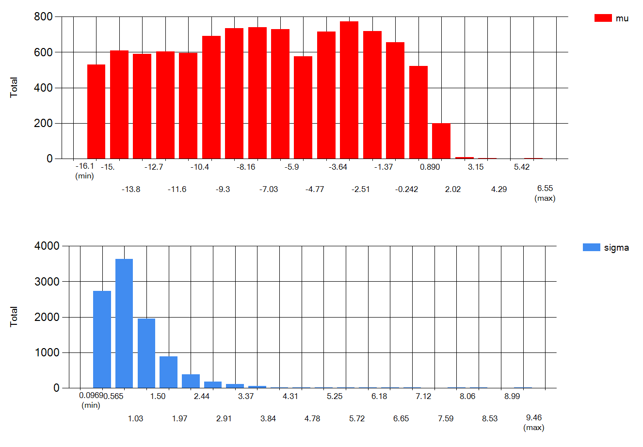
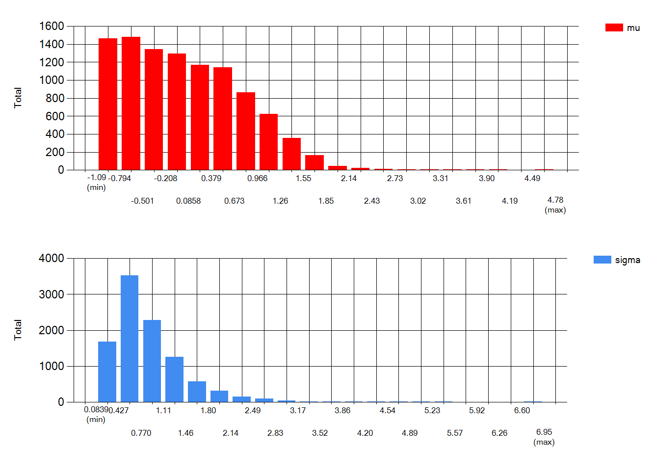
To come back to using expostats with a lot of non detects: the calculation will run but you will observe a very large residual uncertainty because of the lack of info embedded in NDs. This also means that indeed adding one single observed point can change things drastically, beauce one observed point contains a lot more info. Finally lack of information from the data means that the results rely more heavily on the prior assumptions in the calculation engine, so you could see very different results for the same data between tools not using the same set of priors.

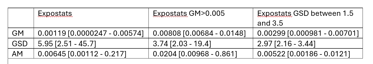
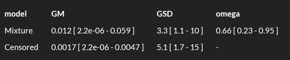
Specifically for IH data, I wouldn’t be to worried by lots of NDs when the LOQ is quite lower than the OEL. However I would be more careful with ND only data when LOQ is rather close to the OEL. As an example, look at what happens when you input <100 3 times in expostats with OEL=100. GM is reported to be anywhere between 10^-7 and 30, GSD anywhere between 1.3 and 10 : we know very little. The BDA chart though suggest there is at most 6% chance that the 95th percentile is above the OEL. However if I change the prior assumptions (e.g. assuming that the true GM cannot be lower than 1 ppm) , these chances increase to 25% (this cannot yet be done in the public expostats).

Trying to get to a bottomline : A high proportion of NDs is OK in Expostats but, especially when the LOQ is close to the OEL, the risk results will depend heavily on internal assumptions. Also RE the difference in likelihood between a range and < : use the range capability of expostats (unique to expostats) whenever you can force the lab to tell you “detected but not quantified” instead of just “not quantified”.

JĂ©rĂ´me

1 Like

Hey Jerome,

Thank you for this detailed response. As you know, I am working on this simulation program and I am running into a unique situation. How does expostats handle data where all of the non-detects are the same value? Like <5, <5, <5. The outputs show non-sensical (to me) low results for the inferential bayesian stats. Frequentist are all NA as there is no variability.

For my simulation program, I am treating any inferential stats from this situation as NA and excluding the results. I am mainly comparing the simulation results to > or <OEL and generating a histogram. Any recommendations on that approach?

Thanks!
Mike

Hello Mike,

The fact that the LOQs are equal does not matter (for the bayesian approach), the important factor is the data are all non detects. Have a look at the figure in my previous answer. Only NDs basically means the likelyhood profile (for the GM) will look like the green curve : the data suggests an upper bound, but all low values are equally likely. A bit simplified this means the entire prior universe (recall the expostats prior for GM is very wide) is equally likely, our lowest possible value being GM as low as OEL/10 000 0000. So the actual posterior distribution will also look somewhat like the green curve. And trying to summarize it with a center and an interval will lead to seemingly nonsensical results.

This does not mean expostats is useless in that situation, because, again refering to the green curve, the right part of it seems useful : we can get usefull upper limits. However point estimates and intervals…less interesting.

Keep in mind though that the exact upper limits might depend on the prior universe, and testing several priors (especially their lower limits) might reassure you.

The all ND case will only become very tough to interpret when the LOQ is close to the OEL. In these situations, playing with the prior seems warranted and might not even lead to a very strong decision.

Testing other priors cannot yet be done in expostats, but can be experienced using our C# prototype : link

Below are direct outputs from this prototype : 3 <5 values with OEL 50

easiest is blue : posterior distribution for log(gsd)=sigma. This is in essence the expostats prior.

in red the posterior for log(gm)=mu. you see the parallel with the green curve above.

The 95%UCL on P95 is 6

Below is what happens when the lower limit on GM in the prior is set to ~ 0.5, which starts to be a bit close to the OEL in terms of a realistic universe of possibilities

The 95%UCL on P95 now becomes 40

In that case, I would conclude that even when assuming the true GM cannot be below 1% of the OEL, the 95%UCL on P95 is below the OEL. IMO this should be a green conclusion.

Does that help a bit ?

Hey Jerome,

Thank you for this, I think it clarifies some things. Is there any value to the point estimates then in these cases?

For example, in the case of <5, <5, <5, my GM point estimate is 0.00036, AM is 0.000789, and 95%ile point estimate is 0.002.

I am simulating the performance of the 95th percentile point estimate, so for any cases like this I am excluding them from the analysis, and only including sims where I get at least one detected value. I’m making this a blanket rule for any criteria to simulate (UTL, UCL of AM, AM, GM, etc.) but maybe that isn’t appropriate and introducing bias? Or maybe it is ok so long as that is explicitly defined for my simulations?

Thanks!
Mike

Trying to answer more practically: In this situation, with expostats, you get a super vague posterior. A point estimate means little, and you can’t even get a value with the frequentist equation.

I faced the same issue when testing the influence of the position of the LOQ vs the OEL. I had a lot of scenarios with >80% non detects.

I chose to report the % of “estimable” situations for the frequentist approach, and the proportion of correct answers, with “non estimable” counted as “incorrect”. For the Bayesian approach, always estimable, I reported the % of correct answers.

With that approach, you can report the real-world performance of the analysis methods in these “dire” situations.

Your approach might bias the analysis if you disregard some generated samples. The ones you keep will come from an unknown distribution, not your original one. I would rather choose something that doesn’t exclude any generated sample, maybe a variation of what I did.

Another approach, since your focus isn’t the treatment of NDs, is to restrict your situation to at most moderate censoring level.

Hello,

In the course of helping colleagues facing a dreafull “all NDs” dataset, I worked on improving the comparative boxplot in tool3 around the idea of showing posterior predictive distributions.

This was also the occasion to graphically show the effect of heavy censorship on the analysis of measurement data.

The result of this small effort is presented here.

Comments welcome !

Hello.

I post here on behalf of Drew Lichty who had a similar “high censorship” issue :

I have input the following samples into expostats Tool 1:

0.036335
<0.008595
<0.008269
<0.007672
<0.006604
<0.009138
<0.010113
<0.006054

I am given the following parameters (my decision statistic is the 95% UCL AM).

GSD: 5.9
AM Point estimate: 0.00642
AM 95% UCL: 0.276

I am wondering why the 95% UCL is so high? I understand that the sample is severely censored, but it still seems quite high to me. I don’t exactly know what is going on “behind the scenes” with censored data, but for comparison, when I input this sample into IHSTAT and transform the <LOD values by LOD/SQRT(2), I am given the following estimates:

GSD: 1.9
AM Point estimate MVUE: 0.009
AM 95% UCL Land’s Exact: 0.018

To me, the IHSTAT 95% UCL seems more reasonable given the sampling data. I am wondering if this is a case of 7 samples <LOD and one sample being quite a high outlier is throwing things off a bit - but still, I would have thought that how expostats handles <LOD values is approximately similar to the LOD/SQRT(2) transformation - such that you wouldn’t get such wildly different estimates for the GSD and UCL 95%.

Because my decision statistic for risk categorization in this case is the 95% UCL I am just a bit concerned as to why they are so drastically different between the two tools.

In my next post are my thoughts and also some sensitivity analyses using the Webexpo prototype (calculations also available in the soon to be released IHSTAT bayes 2.0, and probably also available in 2025/2026 directly in expostats)

First comment : the simplistic LOQ/2 approach give a false sense of “reasonsableness” : with this you replace an unknown quantity with a single value. The answer you get (UCL included) assumes the entered values are true values, not invented. 2 consequences :

  1. variability is underestimated (e.g. if you have only one LOQ and only censored data, there is no variability at all, which is nonsensical except when the agent is truly absent from the worplace.
  2. The uncertainty estimated using frequentist equations is simply false as these equations assume you have provided accurate measurements of exposure.

Now onto the Bayesian methods. As described in this thread and the documents I created, with highly censored dataset, the priors are very influencial so sensitivity analyses are important :

I tested 3 priors :

Expostats prior : GSD from Kromhout et als database, lower bound for GM in this case is 2.10^-9
Expostats prior with lower bound for GM=0.005 (~half the LOQ)
Uniform prior, same as default expostats for GM but GSD assumed between 1.5 and 3.5

Not easy to get a bottomline :slight_smile:

Without your detected results the 3 analyses would suggest very low exposures. But your only detect is fairly high compared to the LOQ, which drives the GSD estimate very high except when we force it to be reasonable. AM being a function of GM and GSD, it is also driven high.

I don’t know the circumstances around this dataset, but I would seek a way to separate the 1st measurement from the rest, or maybe try the “mixture” model I worked on with Igor Burstyn. App. Publication

With your data :

The mixture model is reported to be 1.3 time more likely than the simple censored model (very little evidence). IT suggests a population with 66% zeroes and the rest a lognormal distirbution.

Sorry for not providing a more definitive answer

Cheers