I’m currently trying to replicate the WebExpo models in PyMC. Half learning / half stubborn with picking up R.
I have a ‘working’ model based on the informedvar, however when utilising the data from Section 4.3.3 of the WebExpo report for comparison against different programming languages, I am getting “slightly” different results. Typically, my GM point estimates are slightly lower, and my GSD point estimates are slightly higher.
From what I can suspect, it could be how censored data is handled between your implementation (I suspect) vs how PyMC handles censored data natively. The default censored class doesn’t impute the censored data based on uncensored values, it integrates the censored values out and account though the log-likelihood.
I’m not sure how JAGS approaches this (imputes based on values from uncensored data, or integrates out and accounts on log-likelihood). I have attempted to implement imputation outside the default class however the results are no where as close as below.
It’s either that, or differences between Gibbs and No U-Turn Samplers?
Anyway, here is the data so far. The differences are small enough that at the end of the day, I can’t see the end interpretation being different. But I do like consistency.
If anyone has insight, would be amazing.
Data set:
webexpo_compare_data = ['<25.7', '17.1', '168', '85.3', '66.4', '<49.8', '33.2', '<24.4', '38.3']
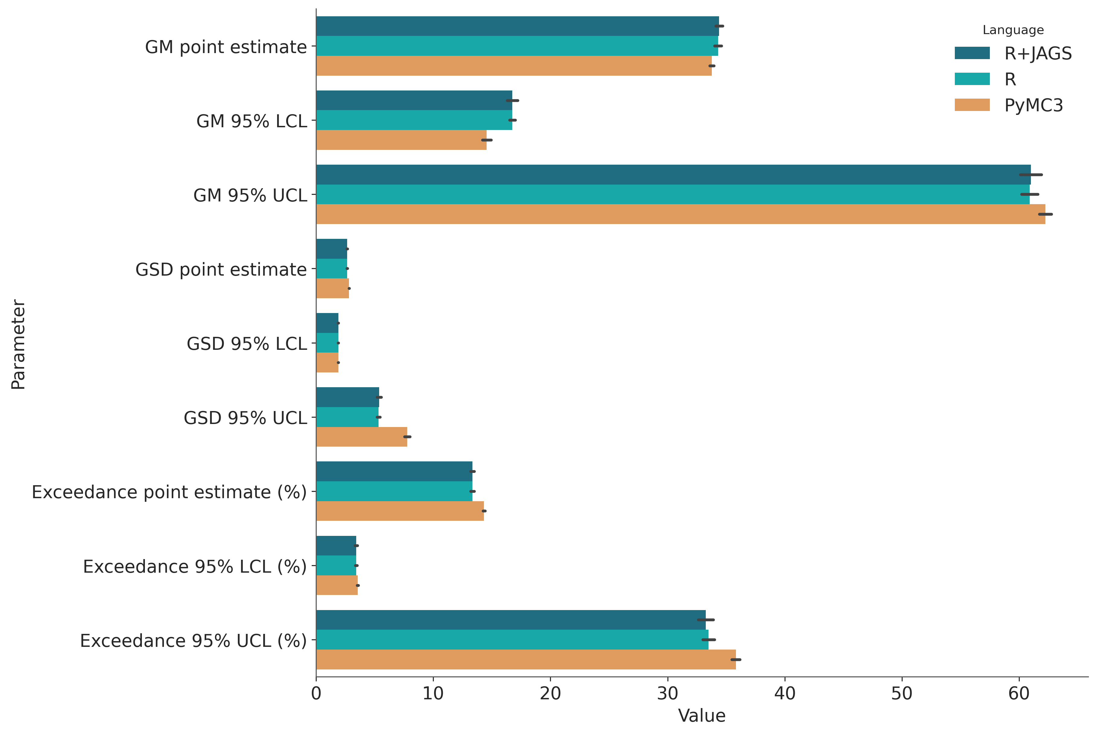
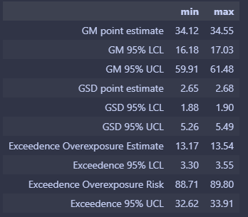
Here are the range of estimates after 50 simulations with the same parameters as the WebExpo report.
- GM point estimate (33.587 33.958)
- GM 95% LCL (14.183 14.934)
- GM 95% UCL (61.723 62.754)
- GSD point estimate (2.802 2.838)
- GSD 95% LCL (1.888 1.902)
- GSD 95% UCL (7.561 8.013)
- Exceedance point estimate (%) (14.233 14.436)
- Exceedance 95% LCL (%) (3.501 3.614)
- Exceedance 95% UCL (%) (35.482 36.178)
Not sure how much my Python is, but here is my model/script.
@dataclass
class CensoredData:
    y: List[float]
    lower_limits: List[float]
    upper_limits: List[float]

def define_observed_lower_upper(expo_data: List[str], oel:float) -> CensoredData:
    y = []
    lower_limits = []
    upper_limits = []

    for value in expo_data:
        if value.startswith('<'):
            # Left-censored
            limit = float(value[1:])  # Extract the numeric value
            y.append(limit)
            lower_limits.append(limit)
            upper_limits.append(np.inf)
        elif value.startswith('>'):
            # Right-censored
            limit = float(value[1:])  # Extract the numeric value
            y.append(limit)
            lower_limits.append(-np.inf)
            upper_limits.append(limit)
        elif '-' in value:
            # Interval-censored
            lower, upper = map(float, value.split('-'))  # Extract the range
            y.append((lower + upper) / 2)
            lower_limits.append(lower)
            upper_limits.append(upper)
        else:
            # Uncensored
            y.append(float(value))
            lower_limits.append(-np.inf)
            upper_limits.append(np.inf)

    # Divide all values by the OEL, excluding infinite values
    y = [value / oel if value != np.inf and value != -np.inf else value for value in y]
    lower_limits = [value / oel if value != np.inf and value != -np.inf else value for value in lower_limits]
    upper_limits = [value / oel if value != np.inf and value != -np.inf else value for value in upper_limits]

    return CensoredData(y,lower_limits, upper_limits)


data = define_observed_lower_upper(webexpo_between_model_data, 100)
with pm.Model() as model:
    # Priors
    mu = pm.Uniform("mu", lower=-20.0, upper=20.0)
    log_sigma = pm.Normal("log_sigma", mu=-0.1744, sigma= 2.5523)
    sigma = pm.Deterministic("sigma", pm.math.exp(log_sigma))
    precision = pm.Deterministic("precision", 1 / (sigma ** 2))

    # Likelihood with censoring
    censored_observations = pm.Censored(
        "y",
        pm.Lognormal.dist(mu=mu, tau=precision),
        lower= data.lower_limits,
        upper= data.upper_limits,
        observed=data.y,
    )

    # Sampling

    trace = pm.sample(
        draws=25000,
        tune=5000,
        chains=4,
        return_inferencedata=True,
        initvals={
            "mu": np.log(0.3),
            "log_sigma": np.log(2.5)
            },
        nuts_sampler='blackjax'
        )